Main Tab
What range of MHz to expect from commonly available VVCs
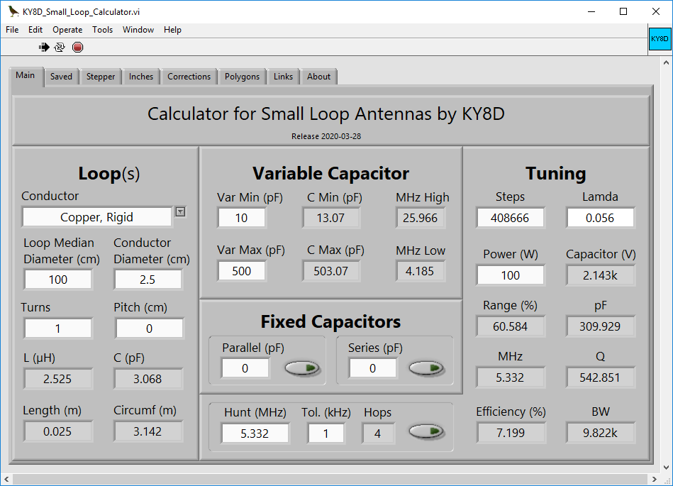
My own (as in yet another) calculator for small-loop transmitting antennas functions differently from all others. Hopefully in a way you will find handy. Focus is chiefly on tuning capacitor. Because once you have either rolled, brazed, or soldered the main loop into a unit whole, there’s no easy way to change that. Also, the loop you can make however you want. Your choices of tuning capacitor, though, can be very limited. Especially if you’re wanting to use a VVC.
Thus I present for your kind consideration my own contestant in an already well-packed arena. Two things it does better than most. Firstly that, for running in a continuous loop, there is no tiresome Calculate button to continually re-click. Secondly is that I have the highest personal confidence in its predictions for loop L (μH) and Cs (pF). This because of employing ultra-modern algorithms recently authored by Robert (Bob) Weaver and David Knight, G3YNH.
Ĝan Ŭesli Starling , KY8D
What's in a name? I too was confused for a long time. But one is a sub-set of the other. And my calculator does both.
The designation magnetic loop specifies a main-loop circumference necessarily smaller than 0.05 λ, according to some. And by no means larger than 0.1 λ, according to many. Only when thus configured does the antenna enjoy deep side nulls.
Larger sizes still work very well. Better, even, if it's radiation efficiency you value most. The self same antenna, when tuned for higher frequencies, gradually loses its side-nulls while gaining higher efficiency. And therein lies a critical difference. Down low it's a magloop; up high it's only a small loop. The same basic antenna structure, but with two very different behaviors.
And magloops came first, their deep nulls important for use in direction finding. You see them in movies about WW2: atop Nazi trucks roaming through streets in search of French resistance cells; mounted on bombers following a radio beacon aimed out of England toward Dresden Germany to direct night-time fire-bombing raids. There is history in the special distinction.
And so, after having twice now suffered (and rightly so) polite harrangues from others much better in-the-know, I bow to the nomenclature gurus, re-naming my program for what truely it is: a calculator for small loop antennas (among which over-category magnetic loops are a particularly venerable sub-set).
The distinction becomes immensely important as circumference approaches λ/4 and larger. Because now it is hardly even a small loop, but increasingly something closer to curled-up dipole with mutually coupled capacitance hats. And still it will resonate. The radiation pattern, however, will by now be growing a lobe. So that unless it's our goal to shine a warming radiation upon worms or birds, then our capacitor will best be mounted at either three or nine o'clock instead of the usual six or twelve.
You’ll need two things for it to run: my *.exe application itself, plus also the interpreter program on which it runs. Kind of like Java that way, except that the Java interpreter is probably pre-installed on your system. The LabVIEW run-time engine will not be.
ky8d.net/free where I give download instructions. ZIP archive software (like 7-Zip ) for extracting the *.exe file to somplace useful prior to trying to run it. Otherwise, Windows will issue dire warnings of an unrecognized app. Once extracted from out of its ZIP archive, however, Windows will know to pass it off to the LabVIEW Run-Time Engine instead.A few features, admittedly, my calculator still lacks. Chief of these is no compensation yet for the loop's nearness to ground. I'm still pouring over several different methods for how to do that. They seem to be in fairly profound disagreement with one another. So I'm not sure yet, which to follow and which to ignore. And so for now ... with some embarrassment ... I still present efficiency numbers for free-space installation. As in quite a bit higher than your own is likely to be. And so, in this one regard, not too very realistic. I will be adding that feature in the fullness of time. That one, along with some others ... just as soon as I can make up my mind which guru it will profit me most to steal from.
It’s an *.exe built on Windows 10 from LabVIEW source code. You can play with it live. In that my aim is for mine to be a bit handier than all the others. Or handy, at least, in a different way. Try it out and let me know what you think.
|
|
Other Tabs: Saved Tab , Stepper Tab , Inches Tab , Corrections Tab , Polygons Tab .
Here are five alternative small-loop antenna calculators. Each gives a somewhat different report. They disagree slightly, not only with mine, but also among one another. All were fed equivalent inputs. These are thumbnails. Click on any to see it larger (and then again for larger still).
|
|
|
|
|
|
My calculator presently does not account for height above ground. I'm working on this. Once I have it nailed, efficiency seems likely to suffer notably for any antenna below one half lambda. As for the slight discrepancy in distributed capacitance, I am using David Knight's formula, whereas some others multiply one dimension by a constant. I am waiting on a reply from DG0KW on his calculation formula. He shows it in red; I'm not clear on why. In the meanwhile, consider my predictions to be for free space.
On first clicking the *.exe icon, the program could come up already running. Look for a black, rightward-pointing arrow at the top left to know that it is indeed running. In the screenshot above, you will see that it shows running. The red stop sign will halt execution, whereupon the black arrow will turn white. Click on the now-white arrow to start execution again.
Right-click on any widget to be provided a menu, then choose Description & Tip to be informed of that widget’s purpose and features.
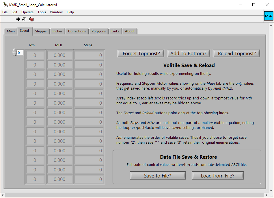
Any frequency which you’ve hunted using Hunt (MHz) on the Main tab, those results will be automatically saved. Likewise you can save any you dial up by hand by choosing Add to bottom. Any frequency saved may be re-load back onto the Main tab, but only from the topmost showing position. Scroll the arrays up and down for puting them into the topmost position. Delete any in th same fashion.
The top left scrolling index indicates only array position (zero based). The first column of the array set shows the order in which runs were saved.
Saved data in the left-hand table are volatile. They will evaporate when stopping the program.
At bottom, however, you have the option to write-to and read-from a tab-delimited ASCII file. Make use of this once you're done experimenting and have results worthy of space on your hard disk. Being tab-delimited pure ASCII, you may name it whatever you like: *.txt, *.dat, even *.csv (although this last is not really proper). May I suggest *.tsv as the suffix mosts truly correct? An advantage will be that MS Excel, in refusing to recognize *.tsv will also decline to corrupt it with extraneous tags ... as otherwise it will be wont to do. To view *.tsv, just open it in any pure-ASCII text viewer.
And if you view Antenna Height (m) in that list, for now please ignore it. It's only there as a built-in place-holder for a feature I'm still working on.
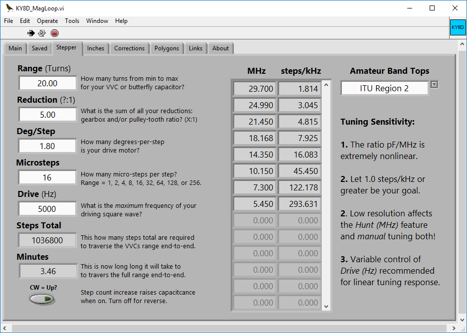
Worry more about frequency tunability at the topmost band more than how long it takes to traverse end-to-end. A table is provided of all tunable bands for your own region. If the top-left array box does not show greater than 1, you need more steps.
Attend to the direction of your stepper motor. Bear in mind, that zero steps might mean either 0 or 100% of your tuning capacitor’s range depending on which way you are planning to orient it if using timing pulleys. Thus either CW or CCW can be selected as the upward-counting direction.
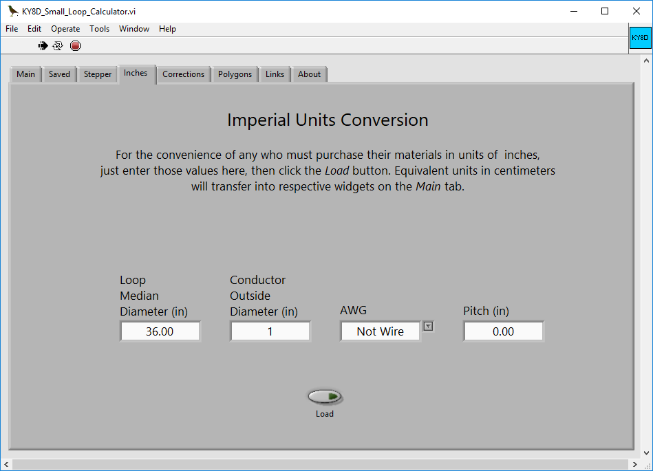
Internally, the calculator is entirely metric. If you own a car newer than 1980, it too is all metric. Even Harley Davidson now designs it’s top-end model entirely metric. But still, in the USA, tubing and pipe can mainly only be purchased in Imperial units. So I offer the Inches tab. Go there to input initial dimensions as inches.
Conductor size may be specified either in inches, or AWG. Selecting any value for AWG besides Not Wire will give the size (in inches) for the selected gauge. Probably you'll not build a small loop out of wire, no matter how heavy. But some people have, and so I accomodate them.
Likewise, if planning to build your loop as a polygon, then output dimensions can be had as either metric (standard) or else in Imperial inches.
The quickest and easiest way of dialing capacitance to the opposite extreme will be to enter an value impossibly high, say 9999999, into the Steps control widget. An override will trim any overshoot back down to its maximum possible limit.
You can also just the the program hunt for desired frequencies.
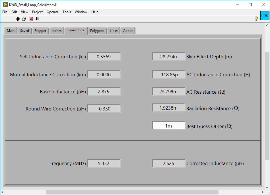
Here mostly you’ll find readouts of the corrections made during calculation of inductance for the main loop.
A solitary input widget allows user-input of any further losses they know of, or simply assume to exist, in units of Ohms. Thus to enter 0.1 Ohms, type in 100m to signify one hundred milliohms.
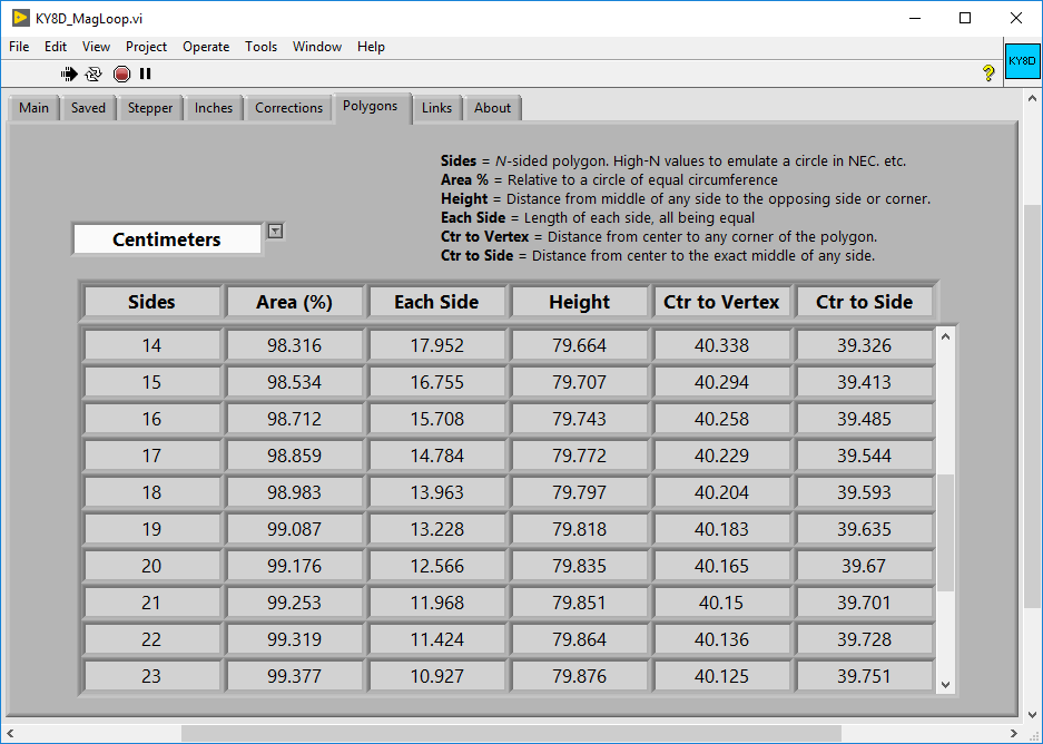
Here you will find, pre-calculated, the geometry of polygons having circumferences of equivalent length to the perfect circle defined on the Main tab. For each is given the area relatvie to aa circle. These measures are provided: length of a side, it’s height with one side flat to the ground (works for both triangles and squares); distance from center to any vertex; distance from center to the middle of any side.
List includes polygons up to 30 sides. This despite copper pipe elbows beyond a 22.5-degree bend being nowhere available. The reason for providing polygonds with more than eight sides is for the convenience of modeling programs, in which, to emulate a circle, polygons are often used. And in such cases, the length of a segment (aka 'side') is constrained by frequency.
Self-explanatory, yes?
You can, if you are extremely stoic, dial in manually capacitance values. On the Main tab, type in any number within the stepper motor’s range. Dial any one digit up or down by clicking beside it and then using the Up and Down arrow keys.
Much faster and far less frustrating is to hunt a frequency instead. Again on the Main tab, type any value into the Hunt (MHz) widget. Find this at bottom center. Then press Enter or else click the button to right. A successive approximation algorithm will take you straight there, nearly always in less than ten hops. Provided, that is, your settings on the Stepper tab are not too coarse. If the hunt algorithm is taking too long, stop it by unclicking the button.
Note also the widget labled Tol. (kHz). If your settings on the Stepper tab are appropriate, leave the tolerance value at 1. Should you insist on setting your stepper motor inadvisably coarse, then in order to hunt any frequency, you must increase the frequency tolerance equally wide.
Most of the established on-line calculators pre-date modern advances in solenoid inductance theory. Instead they are based on methods of calculation which date from the 1920s, with updates no more recent than the middle 1950s. Thus do they harken to a time before the age of computers. It was almost by chance that I myself stumbled upon research into methods of more precise calculation. These date from as recently as 2012 and 2016, authored principally by Robert Weaver, with strong contributions also by David Knight, G3YNH. Their respective PDFs run to hundreds of pages collectively, and are heavily laden with math. No math whiz I, very quickly did I get lost in the intricacies thereof. Importunately, I pestered the authors for clarification. Each responded patiently, and in welcome detail.
Bob Weaver himself hosts an on-line inductance calculator, the new gold standard by definition. His is the one against which I check my own for correctness. I am happy to claim that mine now agrees with that one down to the 3rd decimal place of a single milli-Henry. What small difference there remains is owing to Bob’s calculator employing a Summing algorithm, whereas my own instead makes use of the Sheet-Current method, that together with Round Wire Corrections. My having chose differently had nothing to do with preference, but only on account of my having got one of the two working first. I did that one first as David Knight recommended it, he being the author who whom I had pestered first. In a later email, Bob Weaver affirmed that both methods are equally valid.
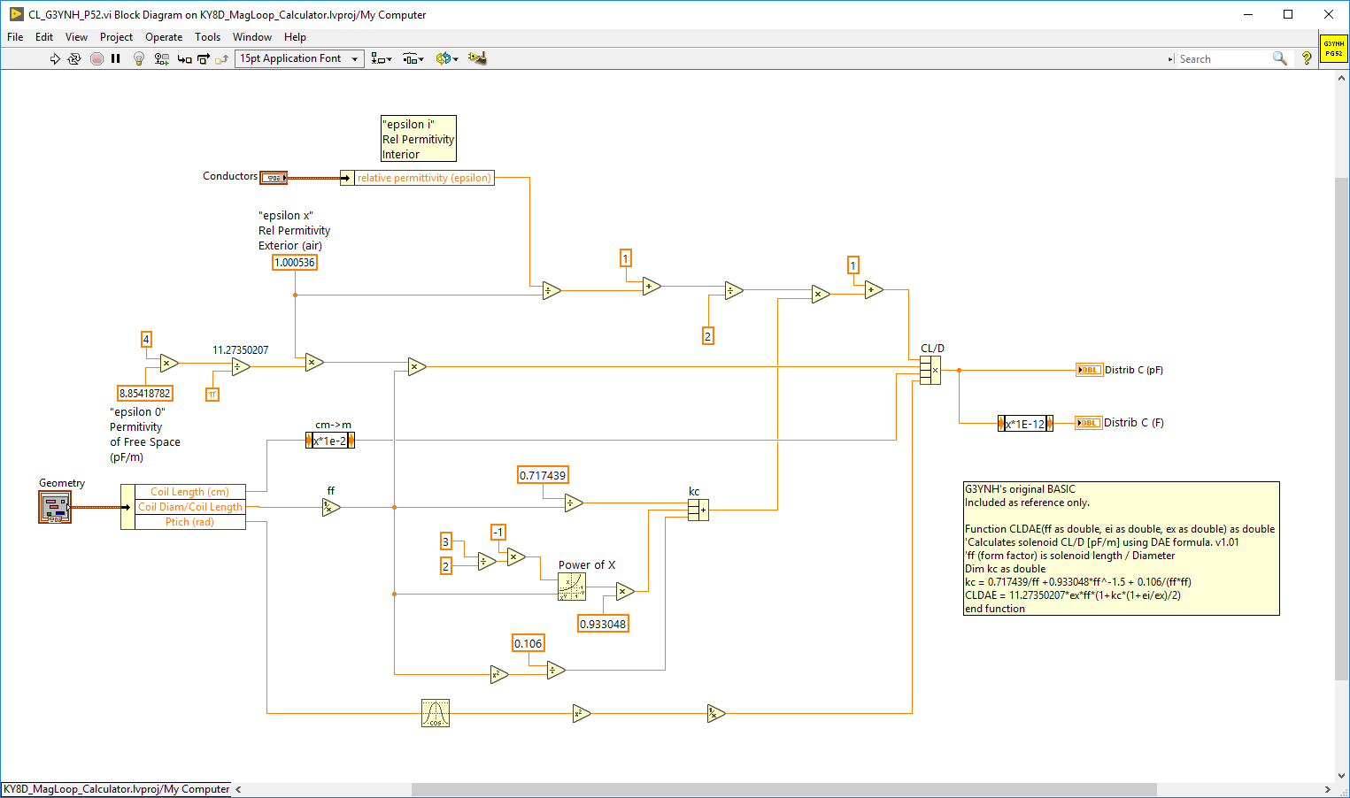
My calculation for Distributed Capacitance of the conductor loop is a trans-code into LabVIEW of an OO Basic function authored by David Knight, titled CLDAE as found on page 52 of his PDF document avaiable here: self-res.pdf . Per said document, this function enjoys a a standard deviation of 2.1%.
Versions of my calculator earlier than 2019-06-06 contained an error in my LabVIEW transcoding of Knight's original function such that reported values were too low, generally below 1pF. As of 2019-06-06 the error has been corrected. Thus will values for Min pF now report higher with the consequence that Max MHz reports lower ... as they should have done formerly. The error was mine. Apology is hereby extended. Current state of the algorithm may be checked here: PNG
Correction for skin effect on inductance is made by subtracting (as per Bob Weaver’s suggestion), the calculated Internal Inductance of the conductor itself. That is to say, the inductance of the wire’s own interior ... that portion beneath the outward-most RF-conducting surface (aka "skin"). Call this the DC Inductance, if you like. At RF frequencies, no current flows there. As far as RF is concerned, there isn’t any ’there’ there. The difference that makes to inductance, however, is so very tiny that Bob suggested I might not find it worth the bother. But where would be the fun in that.
Where skin effect does have a major impact is upon the conductor’s resistance. Let us call it the AC or RF Resistance. We’ve got this fat, thick-walled conductor. But just like a finicky cat, RF energy chooses to only just barely lick the upper-most surface. And so, our apparent cross-section of conductive metal gets thinner and thinner the higher we go up in frequency. Which is why I included tin in the menu of conducting materials ... to demonstrate why we don’t want to plate our copper in tin as a protection against being outdoors in the weather. Better to just paint it instead. Likewise did I include pure aluminum (which no company makes tubing out of) as a comparison against three actual aluminum alloys. The alloys I chose were those which I found for sale on-line. Too often do we hear that aluminum is 63% as good as copper. That would be true if we could buy pure aluminum. But we cannot. And so it’s a myth. Which isn’t to say we can’t use 6061-T6 aluminum alloy, provided we up-size conductor diameter. Do that and aluminum’s greater RF skin depth will help to make up some of the loss. Also, I chose to include silver. Since it might be the case someone’s wanting a small loop for VHF or UHF. In that event, plating with silver would not be a ruinous extra expense.
By email, one user asked whether I apply this correction also to the (assumed hollow) conductor’s interiror surface. I do not. I had not even concieved of this. Somewhere else I had read that no current may be expected along the tube’s interior surface. I wasn't sure whether to credit this, and so it remains a question I still must explore.
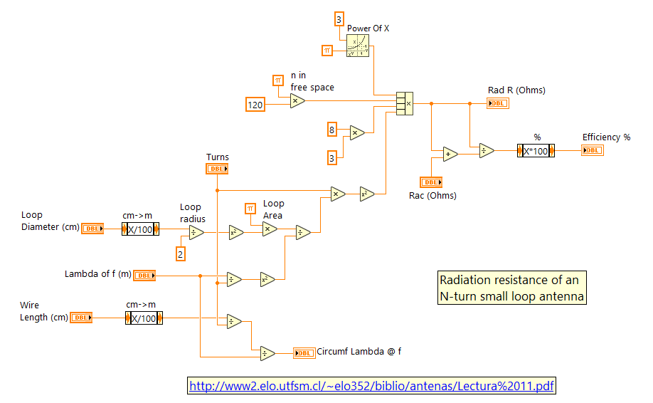
Efficiency I calculate as the ratio of radiation resistance over combined radiation-plus-ohmic resistances. That times 100 to obtain percent. And radiation resistance I calculate according to an equation obtained, not from either Bob or David, but instead from the PDF linked-to below: in equation 11.10; using the free-space constant of 120π. A wholly different formula for Rrad is to be found in the book LF Today, in chapter 7, page 120. Both formulea agree with one another in their results.
By email I was asked whether I calculate Q at the -3dB points of 2:1 SWR bandwidth. I do not. I calculate both at the tuning frequency’s absolute center. Doubtless there are valid arguments for doing it instead at the edges, but so far I find them unpersuasive. Maybe because I'm a CW op, and a Morse code rag-chewer at that. So never for me is it ever the case that I must hop hither and thither in persuit of DX or to rack up a slew of 1-minute contacts.
>Hence the chief goal of my coding this calculator. In building my very own loop (still under construction) I wished to avoid the common lament of so many others, their loops-tuning mechanisms lackig sufficient resolution at the high-frequency end. Pointless, it seems to me, to build a remote-tuning mechanism which after-the-fact proves to still require use of an antenna tuner inside the shack. I just got tired of punching those numbers into other calculators over and over.
Not until that was done did I get around to such further refinements as other calculators already have. I will address this lack more and more as time goes on. For the present moment, however, here’s how things stand.
Presently, this is not dealt with at all. I did have a plan to deal with it, but doubt has now been cast on that method. I'm hoping to take advice from a new source I'm only just now in communication with. Hopefully, he'll steer me straight. Until then, efficiency values remain for free space.
Works, as mentioined above, by way of successive approximation. Actually my second successful attempt at coding such an algorithm. Once before I did a thing very similaar inside of Second Life. Employing SL’s physics engine, my give-away object, Patty the SL Tipping Cow you may enjoy to laugh at on YouTube .
For this calculator the problem was just a little bit more complicated. Capacitance being extremely non-linear to frequency, it’s a bit like navigating via pogo stick up the incline of skateboard half-pipe. Up and down stairs on the inside of that half-pipe. Stairs not of equal rise, but equal instead horizontally. You get the picture.
Whosoever has a dispute with any of my calculator’s results, I vigorously invite that their qualms be made known to me. Provided, that is, ample additional information be likewise cited: contrasting documentation; alternate formulae as examples (newer than 2012); suggestion of a specific math error I might have made. Most helpful would be the presentation of a specific corrective measure. Short of being provided with at least one ofthose, said complaint will fall on deaf ears. I’ll turn my left one ... it’s half way there.
*.ods spreadsheets.*.ods spreadsheets.Because I don’t know either BASIC or Python. And my skill in Perl is quite modest; not up to anything quite this complex. Especially not when it comes to the GUI. Even the math itself is largely beyond my poor understanding. Such are my faults. In LabVIEW however, I am fairly comfortable. Thirteen years now, I have put LabVIEW to use in regular support of my job as a test engineer. So I find myself well able to at the very least faithfully instantiate example equations authored by others. So I here tip my hat to the three maestros cited above (my Aussie bush hat to Owen Duffy).